Multiple correspondence analysis (MCA) is a statistical method. It is applied to generally large tables presenting a set of “qualitative” characteristics for a population of statistical individuals (i.e. “biological” individuals, but also in certain cases institutions, countries, groups, etc.). It extracts what is held to be the most important structuring information from these tables. It provides a synthesis displayed as a graph in which the population studied, on the one hand, and the characteristics detailed, on the other, are distributed in low-dimensional spaces, as straight lines, or more frequently in published work as factorial planes. Similar statistical individuals (and modalities shared by these individuals) are represented on these graphs as points which tend to group together, whilst dissimilarity, on the other hand, results in distance.
This entry provides an overview of the method and its uses in the social sciences. The general elements provided in the first section throw light on questions (notably of terminology) which can give rise to confusion, and briefly examines the origins and dissemination of this method, which was developed by French mathematicians as of the 1960s. It then goes on to explain in what sense and to what extent MCA produces a “synthesis” of the information contained in the tables processed, and presents some useful properties for reading the resultant graphs. Finally, it looks at Pierre Bourdieu’s particular and much noted use of MCA in his social theory. To draw on an analogy he sometimes used, factorial graphs could produce sorts of “geographic maps” of the “theoretical spaces” comprising social fields1.
General elements pertaining to the method and its origins
The term “multiple correspondence analysis” emerged to designate a technique of multivariate statistics which appeared in the 1960s and 1970s, but which may be considered as an extension of an older and better known technique, namely principal component analysis (PCA). PCA is a way of synthesising as a series of “factors” a table of numerical variables for a population of individuals. It has been used at least since the 1940s, notably in psychology. PCA was used for instance by psychologists who, whilst thinking of “intelligence” as a multidimensional faculty, sought to determine a principal factor, similar to the “intellectual quotient”, above and beyond the diverse components they measured in tests (such as conceptual, practical, or affective intelligence, etc.).
MCA, for its part, processes “qualitative” or “categorised” variables, meaning it is of particular interest in the social sciences. Socio-professional category, religious belonging, or gender, for instance, all involve categorisation operations. Each individual is assigned to a single category, where these categories are finite in number, and whilst it may be possible to identify a “modal” category occurring more frequently than the others for a given population, it is not possible to calculate an “average”.
Although the terms “principal component analysis” and “multiple correspondence analysis” are nowadays firmly established, there is nevertheless a degree of terminological uncertainty, especially in the older literature. The expression “factorial analysis” was widely used for PCA, and, by extension, for all techniques--such as MCA--that extracted “factors”. The term “correspondence factorial analysis” (CFA) was also extensively used in French as of the 1970s. Originally it referred to what is nowadays more readily called “standard correspondence analysis”2. This technique is applied to tables of two qualitative variables, such as a “mobility table”. It is very similar to the well-known “chi-square” test. Historically, and mathematically, CFA stands somewhere between PCA and MCA. It is a way of studying the relationship between two variables, and is an extension of PCA conceived as a method for correlation analysis, whilst paving the way to handling qualitative variables.
Jozef Krakovsky, Looking for a countryside (2008)
CFA, and then MCA, underwent major developments in France as of the 1960s, driven by the “French school of data analysis” gathered around the mathematician Jean-Paul Benzecri. This group developed MCA--and coined the term “multiple correspondence analysis”--at a time of rapid progress in computer science (with the group also producing programmes able to conduct “data analysis”). One of Benzecri’s purposes was to take advantage of the new technical possibilities, for the computers of the 1960s made it possible to process “immense datasets previously destined for the flames or else to gather dust” by conducting hitherto unfeasible calculations, such as the diagonalisation of large symmetrical square matrices requiring “data analysis” techniques3. For Benzecri, advances in computer science provided an opportunity for re-founding statistical practice, especially in the human sciences. “Data analysis” struck him as preferable to the ritual analysis of combined tables, for, rather than studying the statistical relationships between variables taken two by two (by projecting causal relationships onto them, often unwarrantedly), such an approach places them within far larger networks of relationships4.
Benzecri argued against the statistical ideas that dominated at that time in the United States and internationally (and which still prevail today). These are bound up with a probabilistic framework and seek to produce models, and are thus based on a large number of a priori hypotheses. Noting that “statistics is not probability”, he mocks statisticians for having “built a pompous discipline with a wealth of hypotheses which are never satisfied in practice”5. He criticises the proliferation of “models forged a priori and then confronted to data in what are called ‘tests’”, arguing that “the model needs to follow the data, not the other way round”6. Given the difficulties encountered in conducting experiments in the humanities, he felt that the way they imported experimental reasoning into their statistical practice was frequently inadequate.
“Data analysis” is based on different principles. It uses algebra and geometry to combat probabilism, and its core ambition--rather than testing models posited a priori--is to determine the structural principles of datasets based on “analysis without a prioris (one should say the synthesis) of multidimensional variables”7. For Benzecri, it is not a matter of doing away with any attempts at modelling, or of giving up on establishing a “hierarchy of causes”, but rather of establishing--as the essential precondition for research--“axes [along which] the masses are aligned”8. Since “science must handle as vast a set of facts as possible, even though imperfectly described, and systematically find by synthesis the true oppositions and gradations”, “multidimensional methods” needed to play the central role ordinarily attributed to probabilistic models or “one-dimensional studies”9. Amongst all the “multidimensional methods” making up “data analysis”, variants on “factorial analysis” are the most important, with classification methods (dividing the statistical population not in a continuous space but into classes) needing to be perceived as “auxiliary”10.

Jozef Krakovsky, Secret painting (2008)
The “French school of data analysis” was particularly active from the mid-1960s onwards. Its techniques were extensively taught at the Science Faculty of the University of Paris, and by the end of the decade young statisticians who had trained in these new methods started introducing them in the French statistical agencies where they were now employed11. Still, Benzecri and his colleagues never taught at the École Nationale de la Statistique et de l’Administration Economique (ENSAE), the INSEE training academy. INSEE, for that matter, was starting to switch over to econometric approaches originating in the English-speaking world. Nevertheless, there were a certain number of people at ENSAE who acted as relays for “data analysis”, especially young administrators who were alert to the fact that it provided an alternative in a statistical world dominated by American norms12. One of them, Michel Volle, started teaching “data analysis” at ENSAE in 1973, going on to publish a book about the method in 1978, which on the strength of its success was republished in 198113.
These young statisticians, in particular those working in organisations active in the humanities, played a significant role in the dissemination of “data analysis”. Mention may here be made of Ludovic Lebart who worked with Benzecri and wrote a textbook for humanities students and researchers that was reprinted several times. In the 1970s, he was part of CREDOC, a research centre counting several researchers (including Nicole Tabard) heavily involved in “data analysis”14. These statisticians often helped sociologists adopting these new techniques. The first article in the Revue française de sociologie to use “correspondence factorial analysis” appeared in 1970, with the method being used as part of a study of a gallery displaying reproductions of paintings15. In 1972 and 1975, an article about the sociology of education and another about farmers’ assets used CFA16. In the mid-1970s, Pierre Bourdieu and the sociologists working with him started to draw on correspondence analysis. As of 1976 correspondence analyses were published on a fairly regular basis in Actes de la recherche en sciences socials, the journal they had just set up. A quick consultation of the Persée website shows that the phenomenon was not specific to sociology, and that over the course of the 1970s the term “factorial analysis” spread (and frequently appeared for the first time) in journals about geography, demographics, rural studies, and--to a lesser degree--history and political science.
In France, most humanities researchers using statistical tools were familiar with CFA and MCA, even those not actually using them. These methods continued to be regularly used in humanities journals as the 1980s, even though some of their novelty had worn off by now and they had become slightly less fashionable. Advances in computer science further boosted their dissemination, as did the increasing availability and number of software programs as of the 1990s, and especially the 2000s. They were admittedly coming into greater competition from the increased importation of methods widely used in the English-speaking world, often associated with a conception of statistics Benzecri opposed. At INSEE in particular, “data analysis” ceded ground in the 1980s (very visibly in Économie et Statistique) and was replaced by more “international” modelling methods. Something similar occurred in sociology, though much later and to a lesser extent, and eclectic forms even emerged that combined data analysis and models based on regression analysis.
But MCA continued to be largely unknown outside France and a few other European countries. Benzecri’s refusal to go and defend his ideas and methods in the English-speaking world no doubt played a part here17. Some of his colleagues sought to boost the popularity of CFA and MCA amongst humanities researchers in the English-speaking world--as did the researcher Michael Greenacre in Spain in the 1980s--whilst French methods of “data analysis” adopted the main statistical software programs. But correspondence analysis continued to be little used in sociology, and with some very rare (and furthermore somewhat anecdotal) exceptions, it was hardly ever referred to, debated, or used in a publication such as the American Journal of Sociology18. But a shift may be observed since the late 1990s, often associated with the work of Henry Rouanet and Brigitte Le Roux to bring the technique to a wider public. In 2004 they published Geometric Data Analysis (with the Kluwer publishing house), and then in 2010 a volume specifically about MCA published by Sage in a collection that was particularly reputed amongst English-speaking “quantitativists” (“Quantitative Applications in the Social Sciences”)19. The international dissemination of the Pierre Bourdieu’s work played a role here. The temptation to reproduce the empirical operations he had performed, particularly in La Distinction, was behind many works conducted outside France, mainly in the 2000s, that resulted in publications deploying MCA20. In the sociology of culture, at least, the use of MCA ceased to be a clearly French specificity as of the second half of the 2000s, being taken up in articles published in English-language European journals such as Poetics and Cultural Sociology21.
A few geometrical properties of MCA
After these general observations about data analysis, it is now possible to go over a few elements that help understand how MCA graphs are produced, and how they are to be interpreted. It is a way of opening up the “black box” of “data analysis” as it were, via which “a set of input data” is transformed into “a visual representation output”22.
In mathematical terms, “factorial analysis” techniques (PCA, CFA, and MCA) are based on fairly abstract algebraic operations. Adopting a geometrical approach has the merit of being comparatively intuitive23. When carrying out factorial analysis with a statistical software program, one has the impression that the software processes a table to produce a visual “output”. The advantage of this method is that it provides a partial representation of an object, in low-dimensional spaces (often a “factorial plane”), where this “object” is equivalent to the table but most of the time can only be represented in a space with a far larger number of dimensions. Presented thus, the transformation carried out by factorial analysis is largely comparable to the problem encountered by drawing or photography (i.e. two-dimensional representations of space) in representing a volume.
Photographing an everyday object in three dimensions involves adopting one viewpoint amongst all the numerous possible viewpoints of non-equal value. Visual riddles based on very simplified drawings (“droodles”) act as sometimes entertaining reminders that certain viewpoints render the represented object unrecognisable. A man wearing a sombrero, shown vertically, may be reduced to 2 concentric circles. In order to make an object recognisable, certain viewpoints are to be privileged. A website providing advice about how to photograph works of art recommends, for instance, that the “plane of the film be perfectly parallel to the plane of the work being photographed, and the object [...] perfectly centred in the frame”24. factorial analysis proceeds with a comparable principle, and statisticians sometimes say that it operates as we do “spontaneously” when, to sketch of camel, we do so in profile, for this is the best way of conveying its “volume” (a camel being big, long, but thin) and its specificity (it would not be possible to make out its two humps with a front-on drawing). In acting thus, we choose not only to place the camel at the centre of the drawing, but also to represent it along what strike us as the best two axes.
To appreciate how factorial analysis proceeds in similar fashion, we can take the very simple case of a PCA performed on two quantitative variables Table 1 shows two numerical values for the socio-professional categories used by INSEE: the percentage of homeowners and homebuyers, and the proportion of members from the category who declared they went to the theatre over the course of the previous twelve months. There are two statistical indicators at the bottom of each column: the (unweighted) average of the variable, and its variance, which indicates its degree of dispersal. The fact that the variance is greater in the second column is due to the fact that the differences in theatre attendance between the categories are clearly greater (being virtually zero for some categories, and above 50% in others) than the proportion of homeowners (which in all cases is somewhere between 40% and 70%).

Table 1. The link between real estate ownership and theater attendance
Table 1 is the equivalent of a graph in which the horizontal axis corresponds to a variable (on graph 2, the proportion of homeowners) and the vertical axis to the second variable. The coordinates of the barycentre (G) of the cloud corresponds to the average rates observed in the various categories (consequently 60.5 on the horizontal axis and 21.5 on the vertical axis). It is possible to calculate the dispersal, or variance, of the cloud, which works out at 397.3, which (excluding the decimal) corresponds to the sum of the variances of the two variables (143.9+253.5=397.4).

Graph 1. The cloud of individuals
A first, simple change consists in centring the object, that is to say in making G the centre of the coordinate system. The coordinates of the points along the axes are then those shown in table 2, that is to say the differences from the average. The value indicated for the proportion of farmers who are homeowners, for example, is no longer 85.9%, but 85.9-60.5=25.4 points. It thus conveys information about the position of the category in relation to the population as a whole. Graph 2, like table 2, provides a way of viewing differences. The cloud has the same form and orientation on graphs 1 and 2, and the axes run in the same directions, they have just undergone a translation.

Table 2.

Graph 2. The centred cloud of individuals
It makes no difference whether it is table 1 or table 2 that is processed using PCA, in both cases the software will “output” the two following graphs:
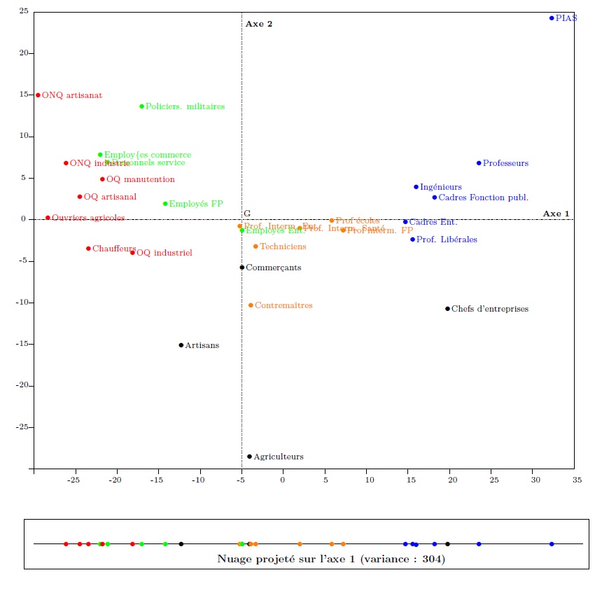
Graph 3. Individuals in the factorial plane

Graph 4. Variables in the factorial plane
It may be seen that the only difference between (“output”) graph 3 and (“input”) graph 2 is a change in the coordinate centre, which has of course preserved the form of the cloud, but changed its orientation and the direction of its axes. Graph 3 is obtained from graph 2 by simply rotating around G (see the animation).
Animation 1.
A particularity of the new coordinate system, however, is that its axes are--in a manner of speaking--ordered. They have been determined in such a way that projecting the cloud of points onto the horizontal axis provides the “best” possible representation of the cloud on a straight line (i.e., in a one-dimensional space).
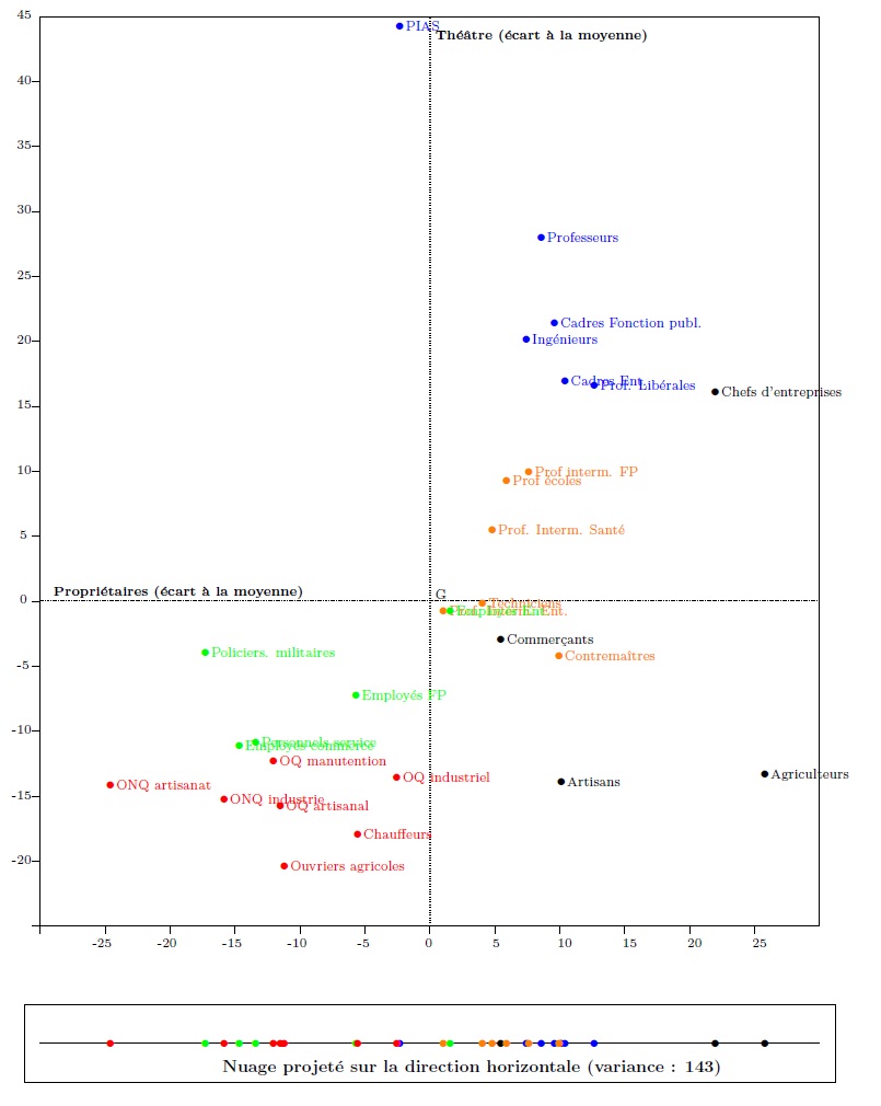
The cloud in graph 3 may be (orthogonally) projected onto all the lines in the plane. If, as in graph 2, the cloud is projected onto the horizontal line (see the cartouche at the bottom of graph 5), this produces a cloud of aligned points, where the coordinates of each point show the proportion of homeowners in the corresponding socio-professional category. The variance of this cloud is that of homeownership rates: 143.9.
Graph 5. Projection onto the horizontal line
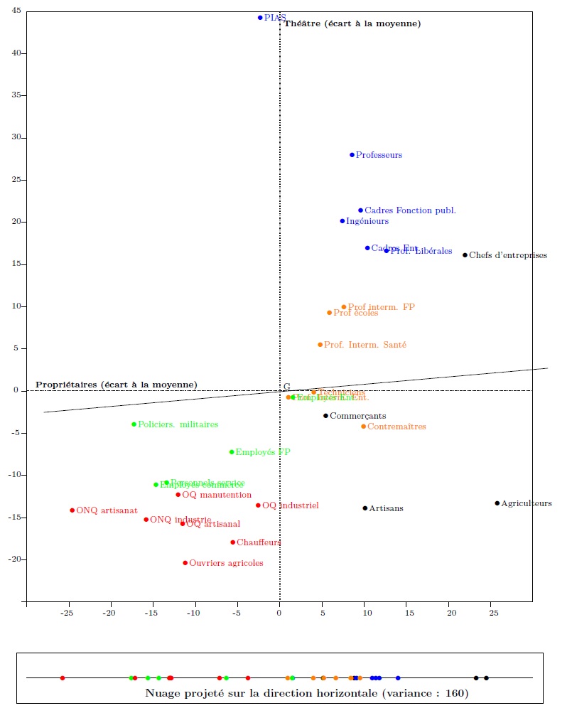
The cloud in graph 2 may be projected onto a line at an angle of 5° from the horizontal. The cloud projected onto this line (graph 6) is slightly more dispersed than the cloud projected onto the horizontal, and it has a variance of about 160.
Graph 6. Projection onto the line at an angle of 5° from the horizontal
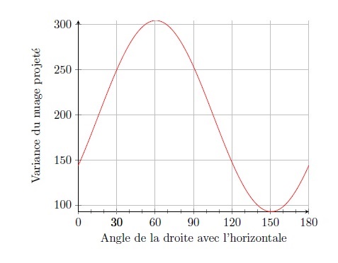
The same operation may be carried out for lines at an increasing angle, through to the line at an angle of 180°, coming back to the horizontal. Over the course of this series of projections (graph 7), the variance of the projected cloud initially increases (up until 61°), and then the tendency is inverted, before increasing once again (after 150°), but without ever reaching the maximum level observed at around 60.58°.
Graph 7. Variation of the dispersal of the projected cloud as a function of the angle of inclination of the line
In a PCA, the line generating maximal variance of the projected cloud constitutes the “first axis”. The variance of the cloud projected onto this axis is the “eigenvalue” of the axis, here 304, amounting to 304.7/397.4≈76.6% of the variance of the cloud in graph 2. Expressed more intuitively, this line is the “principal direction” of the cloud, and is approximately what one would draw on graph 2 to indicate the overall orientation of the cloud (which may be seen to run approximately south-west to north-east). This line maximises the dispersal of the projected cloud, and so maximises the differences between the statistical individuals under study. By projecting the cloud of graph 2 onto this “line of maximal stretch”, the categories furthest apart on graph 2 (i.e. the most dissimilar in terms of the two indicators considered simultaneously) are as far apart as possible in this projection onto a single dimension. To put this differently, the first axis expresses the principal opposition between the socio-professional categories in relation to the two selected variables. It is a sort of one-dimensional indicator resuming the differences relating to the two indicators.

Jozef Krakovsky, My first bike (2008)
At one end of the axis lie the categories which, in table 2, have large negative differences from the average for the two variables under study, in particular all the subcategories of manual workers. The categories at the other end, business managers and “managerial and professional occupations”, display the inverse characteristic (including, in a way, IT professionals and managers: the axis provides a synthesis, and so their comparatively high level of theatre attendance “compensates” their homeownership rate, which is close to the observed average for all categories as a whole). Going from left to right along the axis, from workers to managers, the two variables tend to increase. This is what the second graph produced by the PCA expresses, with the vectors representing the variables being oriented eastwards, that is to say towards the managers.
A PCA does not only determine the principal line, but a new coordinate system including as many axes as the initial coordinate system (or as many variables as the initial table). In the present case it therefore determines a second axis, namely the perpendicular to the first axis passing through G. This second axis relates to a secondary opposition between the categories, as they are progressively further removed from the average profile, positively for one of the variables, and negatively for the other. As the table processed by the PCA here has two dimensions, this second axis is also the final “first factorial plane”, made up of the first and second axis, comporting all the information contained in the table.
If the table had not two but n variables, an identical procedure would need to be imagined in which the cloud of points here represented in graphs 1 and 2 would be deployed in a n-dimensional space. The PCA would determine its principal direction, then (n-1) other axes perpendicular to each other, with the ith axis being the one--of all the lines passing via G and perpendicular to the (i-1) first axes--with variance of the maximal projected cloud.

Jozef Krakovsky, 143-10 (2010)
Understanding MCA entails a further degree of abstraction. As the presence of qualitative variables precludes a representation equivalent to graph 2 (even in a space with a sufficient number of dimensions), an artifice is used, with each variable being transformed into the same number of “dummy variable” as it has modalities. The indicator variable has a value of 1 if the individual is attached to the modality, otherwise a value of 0. This way the population under study may be represented using a cloud of points in a space with as many dimensions as the total number of modalities.
We may take the example of a fairly simple table (and one that is fairly poor in sociological terms) indicating five variables for members of the French government who were in office in January 2016: sex (2 modalities: man or woman); age group (3 modalities: under-45, 45-60, or over-60); an indicator of educational background (3 modalities: ENA/doctorate, IEP or other grande école, or university studies); one relating to declared assets (3 modalities: declared assets of less than €200,000, of between €200,000 and €1 million, and over €1 million); and a final variable relating to the number of times each minister was mentioned in Le Monde prior to the election of François Hollande as president (3 modalities: less than 20 mentions; between 20 and 100 mentions; over 100 mentions). Table 3 gives the first lines of the table (for the five first ministers in alphabetical order).

Table 3. Extract from the table about members of the French government
The table has 33 lines overall, one per minister. Since it is composed of one variable with two modalities and four variables with three modalities, we need to imagine a cloud of individuals which could be represented in a space of 2+3 x 4=14 dimensions. The MCA consists--more or less--in projecting this cloud onto its “principal directions”, which are determined in the same manner as in a PCA. The MCA is thus a form of PCA.
Still, a few further remarks are required. First, since the indicator variables can only assume one of two values, there are only two possible positions on each initial axis. Furthermore, the positions of an individual on the axes associated to the modalities of a given variable cannot be considered as independent, for the way in which nearly all the qualitative variables are constructed results in an individual being attached to just one single modality. Consequently, whilst in an MCA the modalities of qualitative variables play a comparable role to the quantitative variables in a PCA, the cloud of individuals, though theoretically representable in a space with the same number of dimensions as there are modalities, is in fact a cloud with fewer dimensions, and the number of characteristic values (“non-zero” values) is less than the number of modalities (equalling the total number of modalities minus the number of variables).
A final major particularity of an MCA is that it is weighted, with each indicator variable being allocated a weight that increases with its scarcity. In the initial coordinate system the cloud is thus more stretched in the directions associated with rarer modalities, which weighs on the determination of the principal directions. The thing to remember is that an MCA reveals a system of differences, and makes any differences relating to the rarest and most distinctive modalities especially visible. This important effect is not however readily observable in the example of ministers, where the modalities have been constructed in a more or less balanced manner, each corresponding to an approximately equivalent proportion of the population under study (of around one third for each of the 3-modality variables).
The MCA here determines 14-5=9 axes. The statistical programs provide results about the characteristic values (table 4).

Table 4.
The first two axes correspond to 25.7+18.3=44% variance of the cloud. As the variance is necessarily dispersed along a fairly large number of axes, “modified rates” are sometimes calculated which here, for the first two axes, can be as high as 96%, an indicator which may lead us to study the cloud solely via its projections onto the first two axes. Graphs 8 and 9 give the representation of the cloud of modalities and individuals in the first factorial plane.
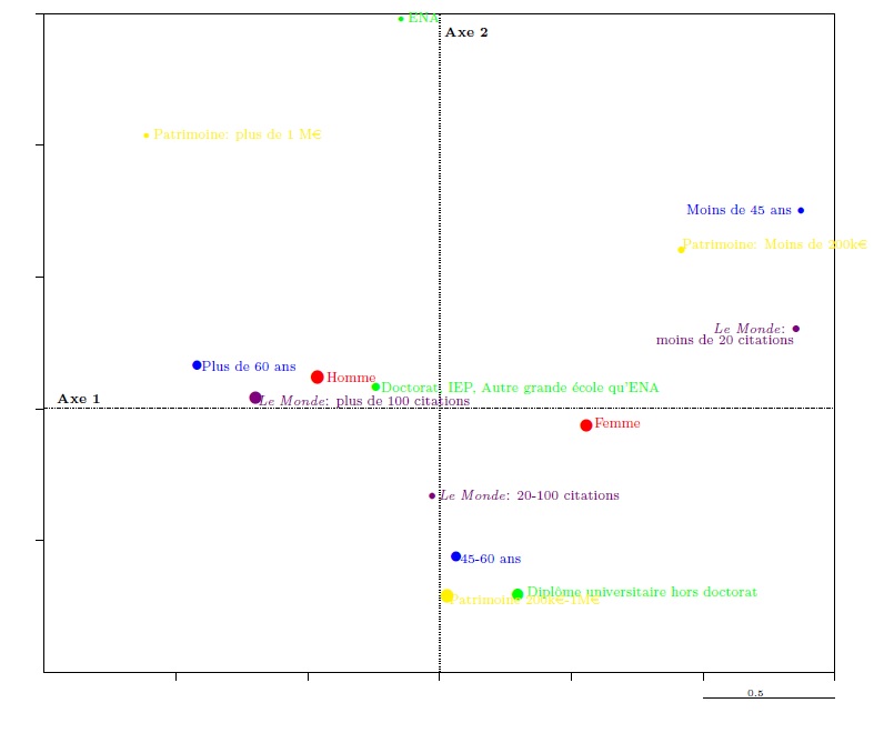
Graph 8. Characteristics of the ministers in the first factorial plane
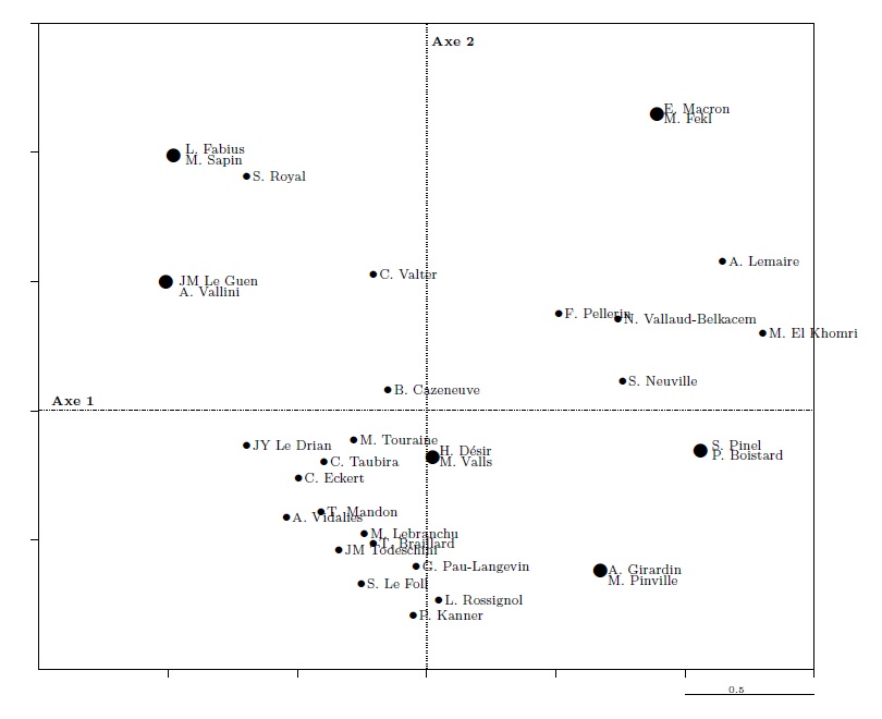
Graph 9. The ministers in the first factorial plane
In graph 8, the first (horizontal) axis shows, on the right of the axis, the age group, asset group, and lowest number of mentions in Le Monde, opposed to the age group, asset group, and largest number of mentions in Le Monde on the left of the axis (it does this using an “interpretative aid” calculated by the software and called the “[modality] contribution to the axis”; see table 5). This first axis opposes, on the left, M. El Khomri, A. Lemaire, S. Pinel, P. Boistard, E. Macron and a few other ministers (who are also young) and, on the right, A. Vallini, J.-M. Le Guen, M. Sapin, L. Fabius, S. Royal, and J.-Y. Le Drian. The most powerful principle of differences (with regard to the variables used in this analysis) is thus clearly associated to age and characteristics that tend to be associated with it, at least among the ministers studied, such as value of personal assets and degree of public notoriety.
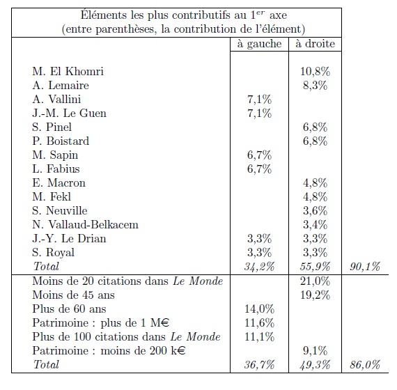
Table 5. Interpretation of axis 1
The second axis relates to a less powerful difference, but one which may nevertheless be detected. It opposes, at the top (see table 6) of graph 8, extremes relating to assets, age group, and especially having studied at the ENA, to average values relating to assets, age groups, and university education (other than doctorates). It opposes ministers of different age who studied at the ENA (E. Macron, M. Fekl, M. Sapin, L. Fabius, and S. Royal) to ministers from the middle age group who did not attend a grande école (or the IEP, and who do not have a doctorate). The analysis cannot be taken particularly far given the low number of variables included in the analysis, but it may be suggested that the axis relates to a difference based on education (and particularly having attended the ENA) and its effect on political careers.

Table 6. Interpretation of axis 2
The example allows us to formulate several properties of MCA graphs which are useful for interpreting them.

Jozef Krakovsky, 82-11 (2011)
The two types of “output” graphs produced by an MCA present the same data same data in two different ways. For example, on the graph of individuals, older ministers are on the same side of axis 1 as the oldest age group in the graph of modalities. The graphs lead us to explore a table (table 3) which may be read line-by-line (individuals) or column-by-column (variables and their modalities).
The graphs of individuals and graphs of modalities in an MCA are united in a barycentric relationship: ministers may be differentiated by age, for example, on the graph of individuals using different colours (graph 10); if we calculate for each age group the barycentre of the points associated with the ministers concerned, the three points associated with the three age groups are spread over space the same way as the points representing the age groups in graph 8 (they are just a bit closer to the origin).

Graph 10. Construction of modality points in the cloud of individuals
This observation also works in the other direction. On the graph of modalities we can calculate the barycentre of modalities attached to one of the ministers (Ségolène Royal for example in graph 11); this barycentre is situated in the same cadran as the point representing the minister in question in graph 9.
Jozef Krakovsky, My red (2007)
We can thus see that if in graph 9 S. Royal is represented by a point that is very close to but slightly lower and further right than that representing L. Fabius and M. Sapin, it is because she only differs from them with regard to one variable, which shifts her slightly south-east (the “woman” point is only slightly removed from the “man” point, and is so in a south-easterly direction).
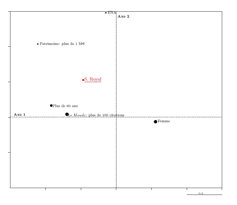
Graph 11. Construction of an individual point in the cloud of modalities
We may also observe that “statistical individuals” are reduced to their statistical profile: L. Fabius and M. Sapin are represented by a single identical point in graph 9 because they are interchangeable in terms of the variables used for the analysis (but constitute two “real” individuals who are evidently distinct and could be represented by very different points if other variables had been used in the MCA).
Proximity between two modalities on the first factorial axes indicates that there is a certain probability of their characterising the same individuals, but this probability can only be estimated by going back to table 3: hence “under-45” and “assets of less than €200,000” are close in graph 8, but 3 of the 8 ministers under 45 years of age declared higher assets.
In an MCA, the modalities of a given variable form a sub-cloud of points always spread out around the centre of the graph: in graph 8, where the variables are identified using different colours, points of a given colour may be fairly close (for sex, in red) or else distant (for education, in green), but they are always to be found in opposing quadrants. This is another barycentric property: the centre of the axes is the weighted barycentre of the points associated to the modalities of a given variable. Consequently, for variables of two modalities, these lie on a straight line passing through the centre and their distances from the centre of the axes is related to their frequency within the population: for sex (graph 11), the relationship dfdh equals the relationship between the number of men and number of women: 17/16=1.0625. It is what is known as the “lever” principle.
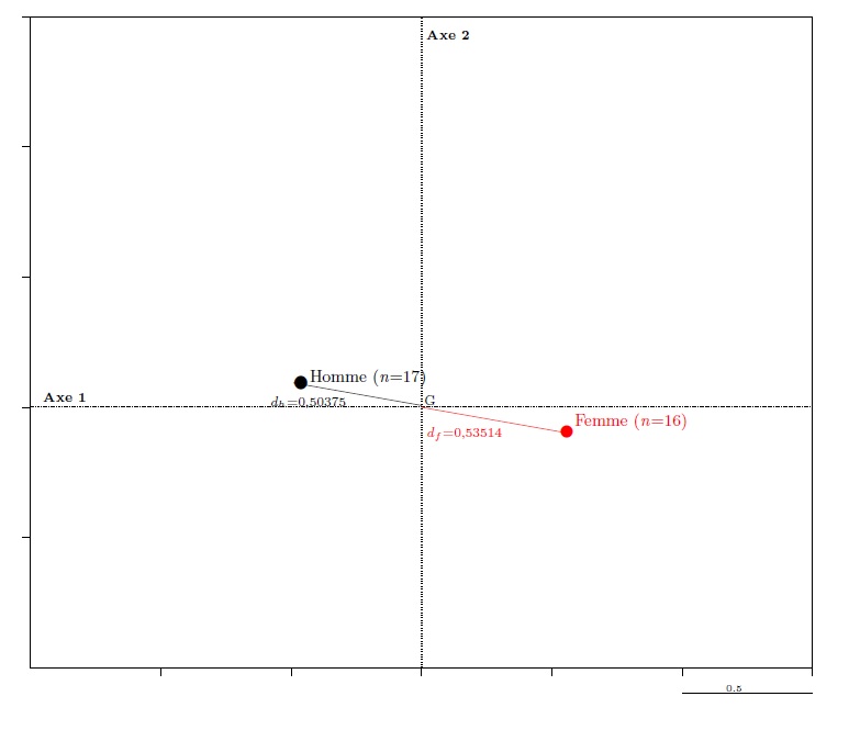
Graph 12. The “lever” principle
Two modalities of a dichotomous variable are thus opposed as a matter of course on all the axes of an MCA. It is consequently not possible to conclude that there is any structural opposition within the population studied unless the modalities lie off-centre from the origin of the axes. The modalities “man” and “woman” on the first two axes indicate that men are slightly over-represented amongst ministers having attended the ENA, elderly ministers, and ministers with high assets, and that women are on the contrary slightly more numerous amongst younger ministers, those mentioned less frequently in Le Monde prior to the election of François Hollande, and so on. Yet the two modalities are fairly close to the centre of the axes, hence sex cannot be considered as a very powerful differentiating principle here, and graph 13 shows that whilst each quadrant is characterised by a fairly clear over-representation of men or women, all of them are “mixed” (compare this with graph 10, where the younger and older ministers are wholly excluded from certain quadrants). This may be due at least in part to the fact that the variables which seem to be the most “structuring” in an MCA are often those with the largest number of modalities.

Graph 13. Cloud of ministers indicated by sex
Once the factorial planes have been interpreted, certain “illustrative” or “supplementary” qualified elements may be projected onto them, where these should not be confused with the “active” elements used to construct the axes. This practice is based on the barycentric properties referred to above.
For example, a supplementary variable distinguishing between ministers and secretaries of state may be projected in the cloud of modalities. The two modalities (see graph 14) are projected near the centre, indicating that the fact of being a minister or secretary of state is only weakly linked to the two major principles structuring the data, even though the probability of being a minister would appear to be (slightly) greater amongst those with the dominant properties (having attended the ENA, being elderly, being a man, etc.).
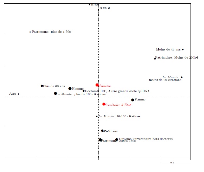
Graph 14. Projection of a supplementary variable
Similarly, it is possible to project additional people in the cloud of individuals, for example the French President François Hollande. He is projected on same point as Laurent Fabius and Michel Sapin, with whom he shares a similar profile.
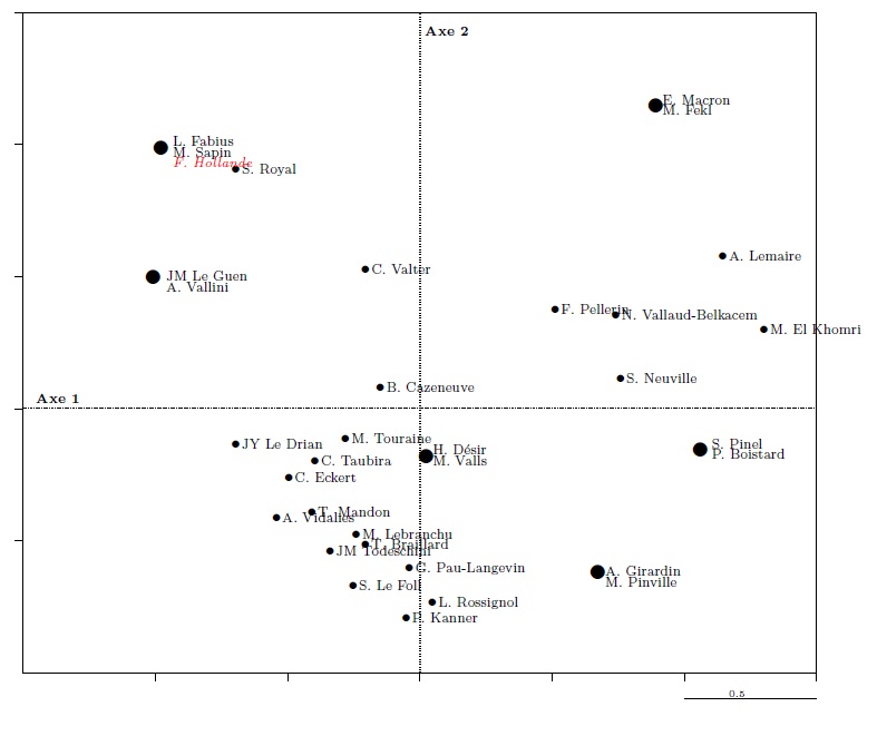
Graph 15. Projection of a supplementary individual
Other statistical methods may be used to expand upon an MCA. The most frequently used is classification, which can be useful for exploiting the results of an MCA so as to construct classes and typologies, by distinguishing several types of ministers (graph 16).

Graph 16. Ascending hierarchical classification of ministers
MCA and the construction of fields
A few brief concluding remarks are in order about the specific use Pierre Bourdieu made of MCA. As Alain Desrosières has noted, the interest Bourdieu expressed for MCA on several occasions is no doubt due to the kinship between his work and that of Jean-Paul Benzecri, both of whom were innovators in their respective disciplines and critical of a form of American imperialism affecting methodology and theory25. They had known each other at the École Normale Supérieure and debated on several occasions, particularly at the 1978 Sorbonne study days26. Yet there is little doubt that Bourdieu did not share all of Benzecri’s views, which were on occasions heavily marked by Thomism and substantialism27. Though he only had affinities with certain tendencies in the “French school of data analysis”, he fully appropriated the tool, and as of his surveys in Algeria with INSEE administrators he took it up into his sociology and ideas about statistical practice.

Jozef Krakovsky, From the series Lines N° 3 (2011)
He came across MCA at the time when “data analysis” was emerging, and never subsequently abandoned it. He drew on MCA in a 1976 article about the “anatomy of taste”, then again in 1978 in a study of business managers, and over the course of the 1980s in his books about academia, the grandes écoles, his survey of housing policy, and, a bit later on, in one of his final studies, about publishing28. His work on the episcopate was also based on an MCA, even though the MCA itself was not included in the publication29. As for the frequently reproduced diagram showing lifestyle attributes and social groups distributed in two dimensions, it does not issue directly from an MCA, even though it is inspired by this method30.
Bourdieu’s use of MCAs is inseparable from his use of the idea of fields. One of the purposes of the MCAs in La Distinction is to build up what he calls “social space”, or sometimes “social fields” or “field of social classes”. The MCAs relating to business managers, academics, senior civil servants, the episcopate, and graduates from the grandes écoles are part of a series of studies he undertook in the late 1970s in various regions of what he increasingly referred to over the course of the following decade as the “field of power”. Not all of Bourdieu’s publications about specific fields include MCAs; some of his works seeking to expand the application of the concept of field (to science, journalism, and law) were not based on in-depth prosopographic investigations31. Although his work on the literary field, which is historical in nature, was started prior to the emergence of “data analysis”, it nevertheless contains certain passages and diagrams which could be compared to virtual or “imaginary” MCAs, as shown by the diagram of the structure of the fields of cultural production, and another diagram showing the overlap between the intellectual field, field of power, and social space (see graph 17)32.
Bourdieu started using MCAs at a time when “data analysis” methods were being taken up, which also coincided with the beginning of the period when the concept of “field” was becoming central to his social theory. It was around 1970 that he started making intensive use of this idea, after rereading Max Weber’s religious sociology in particular33. It may be noted, for that matter, that these re-readings include a diagram based on a series of arrows which seek to represent the system of relationships holding between priests, prophets, sorcerers, and lay people. A few years later he put forward another type of representation of “fields” based on MCA. John Levi Martin has pointed out that whilst Bourdieu was not the only author of a “field theory” in the social sciences to use visualisation tools, in MCA he found one that was particularly appropriate34.
As we have seen, it was MCA that led him to work on systems of differences. MCA focuses on deviations from the mean. It assigns particular significance to rare modalities, that is to say the most distinctive characteristics. It is therefore particularly suitable for the type of relational reasoning advocated by Bourdieu via his concept of field in particular. It processes information, which tends to be collected at the level of the individual, in order to make a structure visible, and thus helps to move away from ways of thinking about the social world which view individuals as the ultimate reality. Instead it looks at “systems of relations”, described by Bourdieu as the “true subject” of social action, where the “major objective for social science” is to ascertain how these systems are constructed.35 Bourdieu pays far more attention to the “clouds of individuals” in factorial planes than do other researchers using MCA. These graphs help apprehend what individuals actually are to his way of thinking--not interchangeable “substances”, but socialised agents situated in relation to one another, and endowed with specific positions and properties.
MCA thus helps to give objective form to the theoretical spaces Bourdieu speaks about in terms of an “invisible reality that cannot be pointed at or touched, and which organises agents’ practices and representations”36. To a certain extent Bourdieu’s use of MCA reflects Benzecri’s hope that factorial analysis would reveal “realities” which had to be “conjectured” before being “recognised as existing”, just as physical quantities such as energy or electric charge once had in the past37. MCA’s capacity to extract “principal factors” from a “sea of data” fulfils the preoccupation of field-based analyses with teasing out the fundamental principles of differentiation, where observation of social life can reveal the virtually unlimited number of principles of differences, but without establishing any hierarchy amongst them. MCA is thus used in La Distinction to establish the volume and structure of capital as fundamental principles shaping cultural tastes, endowed with all the more explanatory power given that so many other potentially associated determinants tend to be invoked (such as age, place of residence, sex, “ethnic” belonging, etc.). But whilst Bourdieu uses MCA’s capacity to extract “principal factors” and thus visualise the “structure of fields”, his purpose is in fact to make full use all of the results generated by MCAs. The distribution of statistical individuals and modalities in factorial planes comes in for in-depth examination in his works. This helps to understand the “poles” present and the power relationships between those endowed with different sorts of capital.

Jozef Krakovsky, From the series Lines n° 7 (2011)
The concept of field is inseparably bound up with the idea of capital in the Bourdieu’s use of MCA. The tables he processes using MCA are nearly always composed of indicators pertaining to the various forms of capital effective in the social space under study for a population of social agents or institutions operating therein. Devising these tables is based on examining forms of capital, for as Bourdieu observes “to construct the social space in the case of France, it was necessary and sufficient to take into account the various sorts of capital whose distribution determines the structure of social space”38. Given that MCA only ever makes it possible to observe the information in the “input” table from a new angle, Bourdieu’s way of proceeding affords a particularly clear illustration of Benzecri’s observation that whilst “data analysis is, in good mathematics, only a matter of looking for specific vectors, the entire science or art of it is to know which matrix to process”39. When Bourdieu makes use of MCA, the construction of the “matrix” raises very substantial questions about the limits and frontiers of fields, and about the effectiveness of various sorts of capital. It tackles this sort of “hermeneutic circle” which, though inherent to statistical work, is very frequently brushed aside in “quantitative” studies in the social sciences40.
The examination of capital continues in the light of the results produced by the MCA, with the first axis nearly always corresponding to the volume of capital, the second to its structure, and the following axes to more secondary principles (such as how the capital was acquired, for example, in La Distinction). MCA as used by Bourdieu helps construct both the structure of the field and the distribution of capital. It is an instrument which takes imperfect and ambiguous information (the active variables are always a series of disparate indicators put together under considerable constraints given that the different forms of capital are unequally objectified in reality, and unequally objectifiable), and synthesises it into more abstract and more pertinent indicators. Only a tool such as MCA can empirically bring out the fundamental forms of capital for which there is no simple indicator (“economic capital”, “cultural capital”, as well as the capital specific to a field, etc.). It is by aggregating and synthesising the active variables that these capitals are made manifest in the MCA process.
The same observation holds true for the “volume of capital”, an expression directly issued from MCA practice. Bourdieu is well aware that in some ways this idea is no more than a statistical artefact. It is highly abstract and difficult to define other than as a variance of the “scale effect”, which is well-known to practitioners of factorial analysis. The “volume of capital” is the fundamental structuring principle that emerges from an MCA when the active variables consist in indicators of various forms of capital. But this idea, which issues from the somewhat obscure aggregation carried out in the “black box” of MCA, also raises very important questions. It provides the empirical underpinnings for the fundamental opposition which would appear to be common to all social spheres, namely that between the “dominant” and the “dominated”. It leads us to enquire into the problem of whether different forms of capital are convertible, as well as the question of whether “capital” conserves any unity above and beyond the various forms in which it specifically transpires.
Thus not only was Bourdieu one of the very first to exploit the geometrical properties of MCA, he also drew profitably on its affinities with relational reasoning and thus used it as a tool to objectify the “theoretical spaces” of fields41. As a tool for construction and objectification, MCA also fed into his ideas about the implications of objectification operations. The only methodological text he wrote about MCA emphasises the value of the method, whilst warning against the risk of “objectivism” inherent to it42. His practice of MCA also no doubt informs the opening chapter of Homo Academicus, which discusses the implications of the objectification operations via which sociology brings out the structure of a space or the distribution of capitals which are only partially objectified in social reality43. Bourdieu’s much remarked use of MCA is in any case a fairly rare case of a social theory closely bound up with a statistical method.
Notes
1
Pierre Bourdieu, La Distinction. Critique sociale du jugement, Paris: Éditions de Minuit, 1979: 189.
2
See Brigitte Le Roux, Analyse géométrique des données multidimensionnelles, Paris: Dunod, 2014.
3
Jean-Paul Benzecri, L’Analyse des données. 2: L’analyse des correspondances, Paris: Bordas, 1973: 8.
4
For an example of this, see what Jean-Paul Benzecri has to say about the then topical issue of the relationship between reading and possessing a television set (L’Analyse des données. 2: L’analyse des correspondances, Paris: Bordas, 1973: 10-12).
5
Jean-Paul Benzecri, L’Analyse des données. 2: L’analyse des correspondances, Paris: Bordas, 1973: 3.
6
Idem, p. 6.
7
Jean-Paul Benzecri, L’Analyse des données. 1: La taxinomie, Paris: Bordas, 1973: 590.
8
Jean-Paul Benzecri, L’Analyse des données. 2: L’analyse des correspondances, Paris: Bordas, 1973: 10.
9
Jean-Paul Benzecri, L’Analyse des données. 2: L’analyse des correspondances, Paris: Bordas, 1973: 16.
10
Jean-Paul Benzecri, L’Analyse des données. 1: La taxinomie, Paris: Bordas, 1973: 590.
11
For discussion of the history of this school and how its methods were disseminated during the 1970s, see Michel Armatte, “Histoire et Préhistoire de l'Analyse des données par J.-P. Benzecri: un cas de généalogie retrospective”, Electronic Journ@l for History of Probability and Statistics, vol. 4, no. 2, 2008; Philippe Bonnet, “Pour une histoire sociale de l’analyse des données”, in F. Lebaron, B. Le Roux (eds.), La Méthodologie de Pierre Bourdieu en action. Espace culturel, espace social et analyse des données, Paris: Dunod, 2015: 21-42.
12
Alain Desrosières, “Analyse des données et sciences humaines: comment cartographier le monde social?”, Electronic Journ@l for History of Probability and Statistics, vol. 4, no. 2, 2008.
13
Michel Volle, Analyse des données, Paris: Economica, 1978 (4th edition published 1997).
14
Ludovic Lebart, Marie Piron, Alain Morineau, Statistique exploratoire multidimensionnelle. Visualisation et inférence en fouille de données, Paris: Dunod, 2006 [4th edition].
15
Yvonne Bernard, “Faits sociaux et jugements de goût”, Revue française de sociologie, vol. 11, no. 2, 1970: 179-196.
16
Lucie Tanguy, “L'État et l'école. L'école privée en France”, Revue française de sociologie, vol. 13, n°. 3, 1972: 325-375; Michèle Salitot-Dion, “Rôle du mariage dans l'accumulation des patrimoines chez les agriculteurs”, Revue française de sociologie, vol. 16, n°. 1, 1975: 59-78.
17
For discussion of the international dissemination of correspondence analysis, see Philippe Bonnet, “Pour une histoire sociale de l’analyse des données”, in F. Lebaron, B. Le Roux (eds.), La Méthodologie de Pierre Bourdieu en action. Espace culturel, espace social et analyse des données, Paris: Dunod, 2015: 21-42; Brigitte Le Roux, Henry Rouanet, Geometric Data Analysis, Dordrech: Kluwer, 2004: 11-13.
18
Ece Kumbasar, Rommey A. Kimball, William H. Batchelder, “Systematic Biases in Social Perception”, American Journal of Sociology, vol. 100, n°. 2, 1994, p. 477-505; David R. Gibson, “Taking Turns and Talking Ties: Networks and Conversational Interaction”, American Journal of Sociology, vol. 110, n°. 6, 2005: 1561-1597.
19
Brigitte Le Roux, Henry Rouanet, Multiple Correspondence Analysis, Thousand Oaks: Sage, 2010.
20
For some references, see: Tony Bennett, Mike Savage, Elizabeth Silva, Alan Warde, Modesto Gayo-Cal, David Wright, Culture, Class Distinction, London: Routledge, 2009; Johannes Hjellbrekke, Olav Korsnes, “Quantifying the Field of Power in Norway”, in K. Robson, C. Sanders (eds.), Quantifying Theory: Pierre Bourdieu, Toronto: Springer Netherlands, 2009: 31–46; Virgilio Borges Pereira, Classes e Culturas de Classe das Famílias Portuenses. Classes sociais e “modalidades de estilização da vida” na cidade do Porto, Porto: Afrontamento/Instituto de Sociologia da Faculdade de Letras da Universidade do Porto, 2005; Annick Prieur, Lennart Rosenlund, Jacob Skjott-Larsen, “Cultural capital today: a case study from Denmark”, Poetics, vol. 36, n°. 1, 2008: 45-71; Lennart Roselund, “Cultural change in Norway: cultural and economic dimensions”, International Journal of Contemporary Sociology, vol. 37, n° 2, 2000: 245-275.
21
For a fairly detailed examination of the use of MCA in the sociology of culture, see Julien Duval, “Multiple Correspondence Analysis”, in D. Inglis, A.-M. Almila (eds.), The SAGE Handbook of Cultural Sociology, London: SAGE, 2016: 255-271.
22
These are the terms used by Jean-Pierre Courtial in “À propos de l'analyse des données. Pour un dialogue entre méthodologue et chercheur”, Revue française de sociologie, vol. 19, n° 4, 1978: 585.
23
For discussion of this point, see Brigitte Le Roux, Henry Rouanet, Geometric Data Analysis, Dordrecht: Kluwer, 2004; Brigitte Le Roux, Henry Rouanet, Multiple Correspondence Analysis, Thousand Oaks: Sage, 2010; Brigitte Le Roux, Analyse géométrique des données multidimensionnelles, Paris: Dunod, 2014.
25
For Bourdieu’s interest in MCA, see for example “Je suis un peu comme un vieux médecin qui connaît toutes les maladies de l’entendement sociologique. Entretien recueilli par Beate Krais”, in P. Bourdieu, J.-C. Chamboredon, J.-C. Passeron, Le Métier de sociologue [1967], Berlin-New York: Mouton de Gruyter, 2005 [5th edition]: xiii-xiv. For American dominance, see Alain Desrosières, “Analyse des données et sciences humaines: comment cartographier le monde social?”, Electronic Journ@l for History of Probability and Statistics, vol. 4, n° 2, 2008.
26
See in particular Jean-Paul Benzecri, “In memoriam: Pierre Bourdieu”, Modulad, n° 35, 2006.
27
On the influence of Thomism, see Karl Van Meter, Marie-Ange Schiltz, Philippe Cibois, Lise Mounier, “History and French Sociological Perspective”, in M. Greenacre, J. Blasius (eds.), Correspondence Analysis in the Social Sciences, London: Academic Press, 1994: 128-137. Jean-Paul Benzecri’s comparatively late text on Cassirer (“Substance et fonction, éléments pour une théorie du concept”, Les Cahiers de l’analyse des données, vol. 3, n° 2, 1978: 239-242), is no doubt in part marked by Bourdieu’s influence, be it direct or indirect.
28
On the anatomy of taste, see Pierre Bourdieu, Monique de Saint Martin, “Anatomie du goût”, Actes de la recherche en sciences sociales, n° 5, 1976: 3-81. This article (together with its MCAs) was reworked in various chapters of La Distinction (Paris: Éditions de Minuit, 1979). On business managers, see Pierre Bourdieu, Monique de Saint Martin, “Le patronat”, Actes de la recherche en sciences sociales, n° 20/21, 1978: 3-82. On academia, see Pierre Bourdieu, Homo Academicus, Paris: Éditions de Minuit, 1984. On the grandes écoles, see Pierre Bourdieu, La Noblesse d’État. Grandes écoles et esprit de corps, Paris:Éditions de Minuit, 1989. On housing policy, see Pierre Bourdieu, Rosine Christin, “La construction du marché. Le champ administratif et la production de la ‘politique du logement’”, Actes de la recherche en sciences sociales, n ° 81/82, 1990: 65-85 (This article was reprinted in P. Bourdieu, Les Structures sociales de l’économie, Paris: Le Seuil, 2000). On publishing, see Pierre Bourdieu, “Une révolution conservatrice dans l’édition”, Actes de la recherche en sciences sociales, n° 126-127, 1999: 3-28.
29
Pierre Bourdieu, Monique de Saint Martin, “La sainte famille. L'épiscopat français dans le champ du pouvoir”, Actes de la recherche en sciences sociales, n° 44-45, 1982: 2-53.
30
This graph, which was already presented in “Anatomie du goût” (Actes de la recherche en sciences sociales, n° 5, 1976: 3-81), was reprinted in La Distinction (Paris: Éditions de Minuit, 1979), accompanied by a note on how it was constructed (see p. 139), and a simplified form of it was included in Raisons pratiques. Sur la théorie de l’action (Paris: Le Seuil, 1994: 21).
31
Pierre Bourdieu, “Le champ scientifique”, Actes de la recherche en sciences sociales, n° 2/3, 1976: 88-104; Sur la télévision suivi de “L’emprise du journalisme”, Paris: Raisons d’agir, 1996; “La force du droit. Éléments pour une sociologie du champ juridique”, Actes de la recherche en sciences sociales, n° 64, 1986: 5-19.
32
"Imaginary" is here to be taken in a meaning akin to "imaginary experiments". Gisèle Sapiro later took up Bourdieu’s analyses of the literary field, producing real MCAs. See for example: G. Sapiro, “La raison littéraire. Le champ littéraire français sous l'Occupation, 1940-1944”, Actes de la recherche en sciences sociales, n° 111, 1996: 3-35; G. Sapiro, La Guerre des écrivains, Paris: Fayard, 1999.
33
See Pierre Bourdieu, “Genèse et structure du champ religieux”, Revue française de sociologie, vol. 12, n° 3, 1971: 295-334; “Une interprétation de la théorie de la religion selon Max Weber”, Archives européennes de sociologie, vol. 12, n° 1, 1971: 3-21.
34
John Levi Martin, “What is field theory?”, American Journal of Sociology, vol. 109, n° 1, 2003: 1-49.
35
Pierre Bourdieu, Raisons pratiques. Sur la théorie de l’action, Paris: Le Seuil, 1994: 54-55.
36
Pierre Bourdieu, Raisons pratiques. Sur la théorie de l’action, Paris: Le Seuil, 1994: 25.
37
Jean-Paul Benzecri, L’Analyse des données. 2: L’analyse des correspondances, Paris: Bordas, 1973: 7.
38
Pierre Bourdieu, Raisons pratiques. Sur la théorie de l’action, Paris: Le Seuil, 1994: 32
39
Jean-Paul Benzecri, L’Analyse des données. 1: La taxinomie, Paris: Bordas, 1973: 590.
40
For discussion of how Bourdieu constructs his tables, see in particular Julien Duval, “L'analyse des correspondances et la construction des champs”, Actes de la recherche en sciences sociales, n° 200, 2013: 110-123.
41
Henry Rouanet, Werner Ackermann, Brigitte Le Roux, “The lesson of Bourdieu’s La Distinction”, Bulletin de méthodologie sociologique, n° 65, 2000: 5-18.
42
This is the text used as a foreword to the article about business managers: Pierre Bourdieu, Monique de Saint Martin, “Le patronat”, Actes de la recherche en sciences sociales, n° 20/21, 1978: 3-8.
43
Pierre Bourdieu, Homo Academicus, Paris: Éditions de Minuit, 1984: 9-52.
Bibliographie
Michel Armatte, 2008, “Histoire et Préhistoire de l'Analyse des données par J.-P. Benzecri : un cas de généalogie rétrospective”, Electronic Journ@l for History of Probability and Statistics, vol. 4, n° 2.
Jean-Paul Benzecri, L’Analyse des données. 1 : La taxinomie, Paris: Bordas, 1973.
Jean-Paul Benzecri, L’Analyse des données. 2 : L’analyse des correspondances, Paris: Bordas, 1973.
Jean-Paul Benzecri, “Substance et fonction, éléments pour une théorie du concept”, Les Cahiers de l’analyse des données, vol. 3, n° 2, 1978: 239-242.
Jean-Paul Benzecri, “In memoriam : Pierre Bourdieu”, Modulad, n° 35, 2006.
Philippe Bonnet, “Pour une histoire sociale de l’analyse des données”, in Frédéric Lebaron, Brigitte Le Roux (dir.), La Méthodologie de Pierre Bourdieu en action. Espace culturel, espace social et analyse des données, Paris: Dunod, 2015: 21-42.
Tony Bennett, Mike Savage, Elizabeth Silva, Alan Warde, Modesto Gayo-Cal, David Wright, Culture, Class Distinction, London: Routledge, 2009.
Yvonne Bernard, “Faits sociaux et jugements de goût”, Revue française de sociologie, vol. 11, n° 2, 1970: 179-196.
Pierre Bourdieu, “Genèse et structure du champ religieux”, Revue française de sociologie, vol. 12, n° 3, 1971: 295‑334.
Pierre Bourdieu, “Une interprétation de la théorie de la religion selon Max Weber”, Archives européennes de sociologie, vol. 12, n° 1, 1971: 3‑21.
Pierre Bourdieu, “The specificity of the scientific field and the social conditions of the progress of reason”, Social Science Information, n° 14, 1975: 19-47.
Pierre Bourdieu, Homo Academicus, Cambridge: Polity Press, 1988.
Pierre Bourdieu, "The Force of Law: Toward a Sociology of the Juridical. Field", Hastings Law Journal, n ° 38, 1987: 805-853.
Pierre Bourdieu, The State Nobility: Elite Schools in the Field of Power, Stanford: Stanford University Press, 1996.
Pierre Bourdieu, The Rules of Art: Genesis and Structure of the Literary Field, Stanford: Stanford University Press, 1996.
Pierre Bourdieu, The Social Structures of the Economy, Cambridge: Polity Press, 2005.
Pierre Bourdieu, "A conservative revolution in publishing", Translation Studies, vol. 1, n°2, 2008: 154-166.
Pierre Bourdieu, Practical Reason. On the Theory of Action, Stanford: Stanford University Press, 1998.
Pierre Bourdieu, On Television, New York: The New Press, 1998.
Pierre Bourdieu, Jean-Claude Chamboredon, Jean-Claude Passeron, The Craft of Sociology, Berlin: Walter de Gruyter, 1991.
Pierre Bourdieu, Monique de Saint Martin, “Anatomie du goût”, Actes de la recherche en sciences sociales, n° 5, 1976: 3-81.
Pierre Bourdieu, Monique de Saint Martin, “Le patronat”, Actes de la recherche en sciences sociales, n ° 20/21, 1978: 3-82.
Pierre Bourdieu, Monique de Saint Martin, “La sainte famille. L'épiscopat français dans le champ du pouvoir”, Actes de la recherche en sciences sociales, n° 44/45, 1982: 2-53.
Pierre Bourdieu, Rosine Christin, “La construction du marché. Le champ administratif et la production de la politique du logement”, Actes de la recherche en sciences sociales, n° 81/82, 1990, p. 65-85.
Pierre Bourdieu, Distinction: A Social Critique of the Judgement of Taste, London: Routledge, 2010.
Jean-Pierre Courtial, “À propos de l'analyse des données. Pour un dialogue entre méthodologue et chercheur”, Revue française de sociologie, vol. 19, n° 4, 1978.
Alain Desrosières, “Analyse des données et sciences humaines : comment cartographier le monde social ?”, Electronic Journ@l for History of Probability and Statistics, vol. 4, n° 2, 2008.
Julien Duval, “L'analyse des correspondances et la construction des champs”, Actes de la recherche en sciences sociales, n° 200, 2013: 110-123.
Julien Duval, “Multiple Correspondence Analysis”, in David Inglis, Anna-Mari Almila (dir.), The SAGE Handbook of Cultural Sociology, London: SAGE, 2016: 255-271.
Johannes Hjellbrekke, Olav Korsnes, “Quantifying the Field of Power in Norway”, in Karen Robson, Chris Sanders (dir.) Quantifying Theory. Pierre Bourdieu, Toronto: Springer Netherlands, 2009: 31–46.
Ludovic Lebart, Marie Piron, Alain Morineau, Statistique exploratoire multidimensionnelle. Visualisation et inférence en fouille de données, Paris: Dunod, 2006.
John Levi Martin, “What is field theory?”, American Journal of Sociology, vol. 109, n° 1, 2003: 1-49.
Brigitte Le Roux, Analyse géométrique des données multidimensionnelles, Paris: Dunod, 2014.
Brigitte Le Roux, Henry Rouanet, Geometric Data Analysis, Dordrecht: Kluwer, 2004.
Brigitte Le Roux, Henry Rouanet, Multiple Correspondence Analysis, Thousand Oaks: Sage, 2010.
Ece Kumbasar, Rommey A. Kimball, William H. Batchelder, "Systematic Biases in Social Perception", American Journal of Sociology, vol. 100, n° 2, 1994: 477-505.
David R. Gibson, “Taking Turns and Talking Ties : Networks and Conversational Interaction”, American Journal of Sociology, vol. 110, n° 6, 2005: 1561-1597.
Virgilio Borges Pereira, Classes e Culturas de Classe das Famílias Portuenses. Classes sociais e “modalidades de estilização da vida” na cidade do Porto, Porto: Afrontamento/Instituto de Sociologia da Faculdade de Letras da Universidade do Porto, 2005.
Annick Prieur, Lennart Rosenlund, Jacob Skjott-Larsen, “Cultural capital today : a case study from Denmark”, Poetics, vol. 36, n° 1, 2008: 45-71.
Lennart Roselund, “Cultural change in Norway: cultural and economic dimensions”, International Journal of Contemporary Sociology, vol. 37, n° 2, 2000: 245-275.
Henry Rouanet, Werner Ackermann, Brigitte Le Roux, “The lesson of Bourdieu’s La Distinction”, Bulletin de méthodologie sociologique, n° 65, 2000: 5-18.
Michèle Salitot-Dion, “Rôle du mariage dans l'accumulation des patrimoines chez les agriculteurs”, Revue française de sociologie, vol. 16, n° 1, 1975: 59-78.
Gisèle Sapiro, “The structure of the French literary field during the German Occupation (1940-1944). A multiple correspondence analysis”, Poetics, 30(5), 2002: 387-402.
Gisèle Sapiro, The French Writers′ War. 1940-1953, Durham: Duke University Press, 2014.
Lucie Tanguy, “L'État et l'école. L'école privée en France”, Revue française de sociologie, vol. 13, n° 3, 1972: 325-375.
Karl Van Meter, Marie-Ange Schiltz, Philippe Cibois, Lise Mounier, “History and French Sociological Perspective”, in M. Greenacre, J. Blasius (dir.), Correspondence Analysis in the Social Sciences, London: Academic Press, 1994: 128-137.


